6 Neural Network Layers
In this chapter we look at the building blocks of a neural network: the layers.
Note: This chapter only partially done, and I’ll add more layers some other day.
What is a layer?
A neural network is basically a function that takes in the input data and produces an output, the prediction. If we zoom into the network, we see that it’s made up of layers. Just like Lasagna, albeit not as delicious. Each layer itself is again a function that takes in data and creates an output, feeding the next layer. Table 6.1 gives you an overview of the most important neural network layers for remote sensing.
| Layer | Effect | Learnable |
|---|---|---|
| 2d convolution | Extract local features | Yes |
| Pooling | Aggregate features | No |
| Transposed 2d convolution | Increase spatial resolution (typically) | Yes |
| Activation | Introduce nonlinearity | No |
You can think of the input of the neural network (e.g., a satellite image) as input features and the intermediate outputs of layers as intermediate features. Mathematically, a feature is a numerical representation of the data. So layers are basically feature transformation functions that change feature from one representation into another.
Layers can be learnable or fixed:
- Learnable layers come with parameters, typically called weights, that are changed during training. An example is the convolutional layer, where the weights of the filters are learnable parameters.
- Fixed layers have no learnable parameters. For example, the ReLU activation layer just applies a non-parameterized function to the inputs.
An over-simplified convolutional neural network would chains layers sequentially:
Input -> 2d convolution -> pooling -> fully connected -> sigmoid
While overly simple, this architecture shows how information flows through layers:
- The 2d convolution layer extracts local spatial patterns like, for example, edges (depending on what it has learned).
- Pooling typically reduces the spatial resolution and aggregates information.
- The fully connected layer mixes feature across the image.
- The sigmoid function squashes the score into the [0,1] range.
Mathematically, we can express the sequence of layers as a nested function:
\[f(X) = f_{\text{sigmoid}}(f_{\text{fc}}(f_{\text{pool}}(f_{\text{conv2d}}(X))))\]
After each layer, we get an abstract representation of our data, which we can call (intermediate) features and become input to the next function.
2d convolution
Extract local features.
2d convolution is the most important layer for remote sensing – it extracts local patterns from image-like data and represents the images with new features. You can think of 2d convolution as a function that takes in a satellite image, or it’s already transformed representation, and computes new channels. These channels are sometimes called feature maps, which I think is a good name.
2d convolution is defined by a kernel that “scans” the input to create new features. This kernel scanning has some similarities to satellites or aircraft scanning the Earth. The kernel is represented by a \(K \times K\) matrix. A common choice is \(K=3\). It’s possible to have rectangular kernels like \(4 \times 2\), but I focus on square kernels for simplicity and because most explanations generalize to rectangular kernels. The input to a convolutional layer not only has spatial dimensions, but also a feature dimension: this could be, for example, 3 RGB channels or 64 output feature maps from the previous layer. Let’s call this dimension \(D\). That means to transform the input features to a new output feature map, we need a weight tensor of dimension \(K \times K \times D\), also called a filter or kernel stack. A filter is a linear projection of the \(D\) input channels into a new channel. A 2d convolution layer contains \(D'\) filters with typically \(D' > D\), so that we get more features after the 2d convolution. The number of filters directly translates into the dimension of the output features.
Filters in remote sensing, such as low pass filters, work quite similarly to 2d convolution. The big difference in deep learning is that 2d convolutions are learned operations, while image filters in remote sensing typically have fixed kernels, such as Gaussian filters.
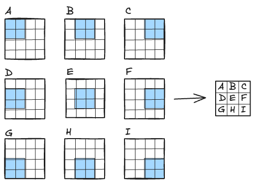
Let’s have a look at how the convolution operation works. Basically, the filter “sweeps” over each part of the image and we multiply the filter weights with the respective “receptive field”, which is the part of the input tensor covered by the filter. This creates one number. We repeat this by moving the filter along the spatial dimensions and, multiplication by multiplication, create a new so-called “feature map”. In Figure 6.1, we sweep with a \(2 \times 2 \times 1\) filter with a step size of 1 (stride=1).
Besides the kernel dimensions, these hyperparameters control the 2d convolution:
- The stride is the step size. In theory, you can set different strides for latitude and longitude. Increasing the stride decreases the spatial output size.
- The padding controls how many rows/columns of 0’s we add to the margin of the input before applying the convolution. The more padding, the larger the spatial output dimensions. A special case is the option of “same” padding, which is just the right amount of padding for the selected kernel size and stride to ensure that input size equals output size.
- The dilation parameter interweaves rows and columns of 0’s into the kernel. This increases the kernel size while keeping the number of trainable parameters the same.
Imagine you have a satellite image of size \(3 \times 3 \times 2\) where the two bands are NDVI and NDWI (see Chapter 3), or simply red and blue channels.
\[ \textbf{Input } X \in \mathbb{R}^{3\times 3 \times 2}:\quad X^{(1)}=\begin{bmatrix} 1 & 2 & 3\\ 4 & 5 & 6\\ 7 & 8 & 9 \end{bmatrix},\qquad X^{(2)}=\begin{bmatrix} 0 & 1 & 2\\ 1 & 0 & 1\\ 2 & 1 & 0 \end{bmatrix} \]
For the convolution, we need a filter. We use a \(2 \times 2\) kernel, and since we have 2 input features (bands), we need a stack two kernels to create a \(2 \times 2 \times 2\) filter. Normally, each filter also has a bias term added to the output, but for simplicity, I’m skipping it here.
\[ K^{(1)}=\begin{bmatrix} 1 & -1\\ 0 & 2 \end{bmatrix},\qquad K^{(2)}=\begin{bmatrix} 2 & 0\\ 1 & -1 \end{bmatrix} \]
With multiple input channels, the general formula is:
\[ Y_{i,j}=\sum_{c=1}^{2}\sum_{u=1}^{2}\sum_{v=1}^{2} X_{i+u-1,\,j+v-1,\,c}\,K^{(c)}_{u,v} \]
\[Y_{1,1} = (1\cdot1 + 2\cdot(-1) + 4\cdot0 + 5\cdot2) + (0\cdot2 + 1\cdot0 + 1\cdot1 + 0\cdot(-1)) =10\]
\[Y_{1,2} = (2\cdot1 + 3\cdot(-1) + 5\cdot0 + 6\cdot2) + (1\cdot2 + 2\cdot0 + 0\cdot1 + 1\cdot(-1)) = 12\]
\[Y_{2,1} = (4\cdot1 + 5\cdot(-1) + 7\cdot0 + 8\cdot2) + (1\cdot2 + 0\cdot0 + 2\cdot1 + 1\cdot(-1)) = 18\]
\[Y_{2,2} = (5\cdot1 + 6\cdot(-1) + 8\cdot0 + 9\cdot2) + (0\cdot2 + 1\cdot0 + 1\cdot1 + 0\cdot(-1)) = 18\]
\[ Y=\begin{bmatrix} 10 & 12\\[4pt] 18 & 18 \end{bmatrix} \]
For a deeper understanding of convolution, I highly recommend reading Dumoulin and Visin (2018) or visiting this interactive convolutional neural network tutorial.
Pooling
Locally aggregating feature signals.
Pooling is a spatial aggregation operation and has the same hyperparameters like 2d convolution: a kernel, stride, padding, and dilation. In addition, we have to decide how values in the kernel are pooled: It’s typically either the maximum or the average. Just like 2d convolution, the pooling operation “sweeps” across the spatial dimensions and creates a new output image, typically with much lower spatial resolution, which is quite similar to what is shown in Figure 6.1. But in contrast to 2d convolution, we do this operation individually for each input feature map. That means when we have \(D\) input feature maps, we again get out \(D\) feature maps with reduced spatial dimensions. You can see each input feature map as a measuring some abstract concept. Since the max pooling operation only forwards the largest value it’s like forwarding only the strongest signal while reducing the spatial resolution.
\[ X = \begin{bmatrix} 1 & 3 & 2 & 4 \\ 5 & 6 & 7 & 8 \\ 9 & 2 & 0 & 1 \\ 4 & 3 & 5 & 2 \end{bmatrix} \]
Max pooling with a \(2 \times 2\) kernel and stride\(=2\) produces a \(2 \times 2\) output:
\[ Y = \begin{bmatrix} 6 & 8 \\ 9 & 5 \end{bmatrix} \]
Pooling is a fixed operation, meaning there are no learnable weights involved. You typically find pooling layers right after convolution layers: 2d convolution creates new spatial features, and pooling aggregates them. By repeated convolution+pooling, the neural network can express more and more abstract features while step-by-step removing the spatial dimensions. A learnable alternative to pooling is 2d convolution with a stride>1 which also has a spatial reduction effect.
Transposed 2d convolution
Increase spatial resolution.
Transposed convolutions are convolutions run in reverse. A bit like rotating a telescope and looking into it from the other side: Instead of magnifying objects, they now look smaller and further away. Let’s take a 2d convolution that turns a \(4 \times 4\) image into a \(2 \times 2\) image: this operation’s transposed convolution turns \(2 \times 2\) images into \(4 \times 4\) images, see Figure 6.2. Most deep learning libraries implement transposed convolutions so that setting the hyperparameters the same as for the 2d convolution makes them a matching pair. For example, a convolution with stride=2 halves the spatial resolution; the matching transposed 2d convolution with stride=2 doubles it again. Transposed convolutions are sometimes also called “deconvolution”, but this is a misnomer as the term “deconvolution” means the exact inverse operation of a convolution, but transposed convolutions don’t recover the exact values.
The purpose of transposed convolutions is learnable increase in spatial resolution. That’s why you find them in architectures for tasks where an increase in spatial resolution is required often followed after a feature bottleneck:
- Semantic segmentation
- Super-resolution of satellite images
- Image reconstruction tasks
Transposed convolution can produce artifacts, the checkerboard patterns. Alternatives are upsampling + convolution, for example used in U-Net, see Chapter 8.
![]()
Instead of transposing a convolution, you can always find a direct convolution that emulates the transposed. However, this may involve adding rows and columns of zeroes to the input and is therefore less efficient.
Activation functions
Enable the network to approximate complex functions by introducing nonlinearity.
Many layers are linear: convolution, transposed convolution, fully connected layer. And if we would combine linear layers, the output would simply be a linear function of the inputs – too limiting. That’s why it’s crucial to insert nonlinearities into the network, which is done with activation layers. The activation layer is just an element-wise application of a non-linear function. The most common pick for this function is ReLU, which stands for Rectified Linear Unit and is defined like this:
\[ relu(x) = \max(0, x)\]
This function sets all negative values to zero. That’s it. Enough to make the neural network nonlinear. There are many alternatives, with tanh and sigmoid being more old-school ones and Leaky ReLU and GELU being more modern ones. They all have the same job of making the output nonlinear.
For classification tasks, the last layer is often an activation layer. This last layer has a different job: It squashes the output between \([0,1]\) – something resembling a probability. To achieve this, many architecture use the softmax function:
\[ \text{softmax}(x_i) = \frac{e^{x_i}}{\sum_{j} e^{x_j}} \]
It transforms a vector of raw feature values \((x_1, \dots, x_K)\) into a probability distribution over \(K\) classes. Most nonlinear functions (ReLU, tanh, GELU) act element-wise. Softmax is different: it couples all the outputs of a layer to normalize them into a probability distribution.
While softmax is often applied when making predictions with a classifier, during training it might not be used but the cross-entropy loss may be applied directly to the last layer.
Notable Mentions
Note: This chapter only partially done, and I’ll add more layers some other day.
- Dropout
- Pyramid Module
- Concatenation
- Batch Normalization
- Attention Mechanism
- Fully connected layer
- 1D convolution
Parts of this chapter draw inspiration from the “Little Book of Deep Learning” François (2023) which I highly recommend as a short reference book for deep learning. It’s free and the PDF is smartphone-sized for all of us geeks learning about deep learning on our phones.