import os
import random
from glob import glob

import numpy as np
import matplotlib.pyplot as plt
from PIL import Image

from sklearn.model_selection import train_test_split, RandomizedSearchCV
from sklearn.metrics import (
    accuracy_score,
    precision_recall_fscore_support,
    confusion_matrix,
    ConfusionMatrixDisplay,
)

from xgboost import XGBClassifier


import torch
import torch.nn as nn
import torch.optim as optim
from torch.utils.data import Dataset, DataLoader
from torchvision import transforms
import torchvision.transforms.functional as TF
from torchvision.models import resnet18, ResNet18_Weights

from tqdm import tqdm

# Ensuring reproducibility
seed = 42
random.seed(seed)
np.random.seed(seed)
torch.manual_seed(seed)
if torch.cuda.is_available():
torch.cuda.manual_seed_all(seed)7 Image-wise Land Cover Classification
In this use case, we will train two different models to classify land cover from satellite images: Both a “traditional” machine learning approach (xgboost) and a deep learning approach (ResNet-18).
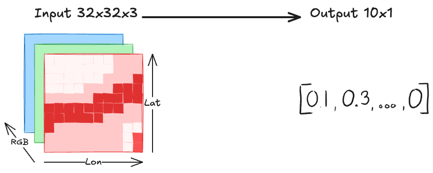
The prediction task
The goal is to predict land cover from satellite images. In this use case we get one land cover label per image, meaning an entire images may be classified as crop or river. This has some immediate drawbacks, because there might be more than one class shown on the image. However, such a rough land cover classifier may still be useful for, for example, filtering satellite images. Having just one label per image makes this task a classic classification task: An image goes into the model, and we get out a score per class or one class as the chosen one. This classification task is visualized in Figure 7.1.
The EuroSAT dataset
We use the EuroSAT data (Helber et al. 2019, 2018a) which contains 27k images from Sentinel-2, covering 10 land cover classes. The dataset is specifically designed for training land use and land cover classification models. EuroSAT comes in two flavors: RGB (size is 95 MB) and multi-band (2.1 GB). We will use the simpler RGB representation, meaning the images have the 3 channels red, green, and blue.
Each image is classified into one of 10 classes:
- Annual Crop (3000 images)
- Forest (3000)
- Herbaceous Vegetation (3000)
- Highway (2500)
- Industrial (2500)
- Pasture (2000)
- Permanent Crop (2500)
- Residential (3000)
- River (2500)
- Sea, Lake (3000)
With 2-3k images per class, it’s a quite balanced dataset. This makes training a classification model certainly easier, but whether it’s suitable for your use case depends a bit on the distribution of the classes in your application.
You can download the data from Zenodo (Helber et al. 2018b). It comes with an MIT license. EuroSAT is a bit like the Iris data 1 of remote sensing – meaning it’s a heavily used example, because it’s an easy-to-use dataset since there are no missing data and you can achieve a high accuracy.
First, let’s import all the libraries that we will need for this use case.
Let’s visualize one image per class from the EuroSAT data. The result is Figure 7.2. You can already see the limitations of image-wise classification here: For example the river satellite image also shows forest.
data_dir = 'data/EuroSAT_RGB/'
label_names = sorted(os.listdir(data_dir))

plt.figure(figsize=(15, 10))
for i, label in enumerate(label_names):
    filename = os.listdir(os.path.join(data_dir, label))[0]
    path = os.path.join(data_dir, label, filename)
    img = Image.open(path)
    plt.subplot(4, 5, i + 1)
    plt.imshow(img)
    plt.title(label)
    plt.axis('off')

plt.savefig('./images/landcover-examples.jpg', dpi=300)
plt.tight_layout()
plt.show()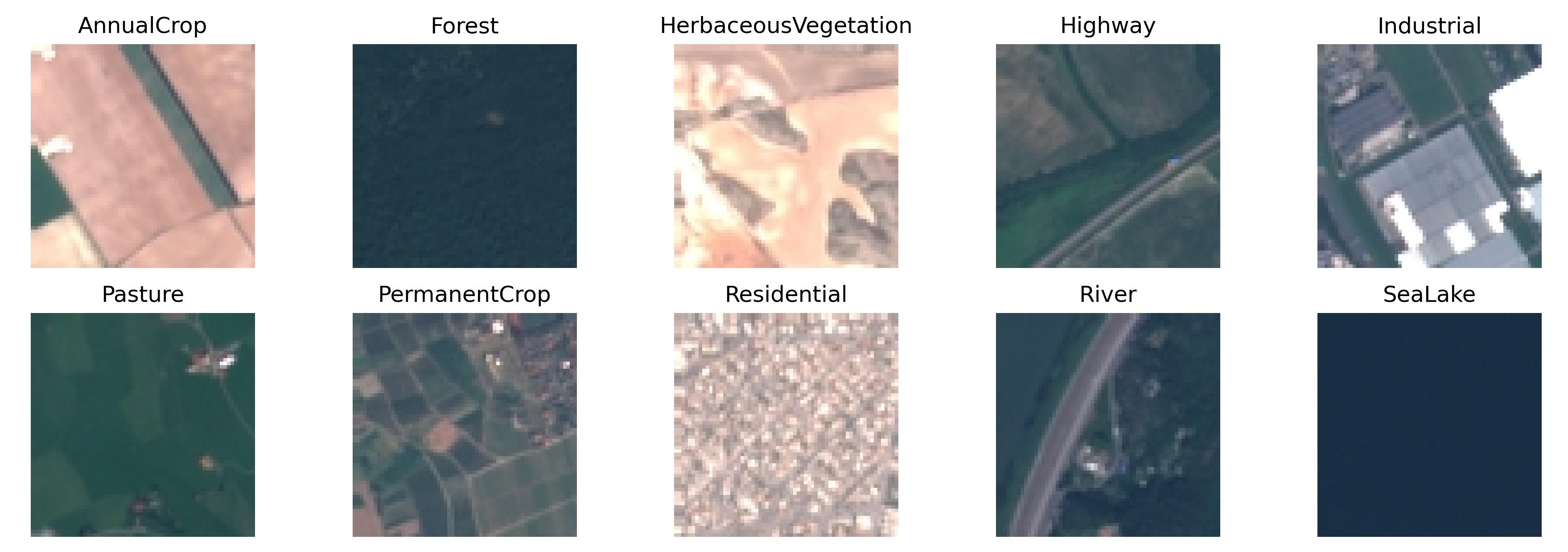
Our models, however, will not work with the image as we see it, but the inputs are the RGB channels. To visualize the input data, let’s have a look at the highway image again. Figure 7.3 shows that the highway image consists of three channels (or bands), which are red, green and blue. If we combine all three colors, we get the full image.
label = label_names[3]
path = os.path.join(data_dir, label, os.listdir(os.path.join(data_dir, label))[0])
img = Image.open(path).convert("RGB")
channels = img.split()
titles = ["Original", "Red", "Green", "Blue"]
cmaps = [None, "Reds", "Greens", "Blues"]

plt.figure(figsize=(10, 6))
for i in range(4):
    plt.subplot(1, 4, i + 1)
    plt.imshow(img if i == 0 else channels[i - 1], cmap=cmaps[i])
    plt.title(titles[i])
    plt.axis('off')

plt.tight_layout()
plt.savefig('./images/landcover-rgb.jpg', dpi=300)
plt.show()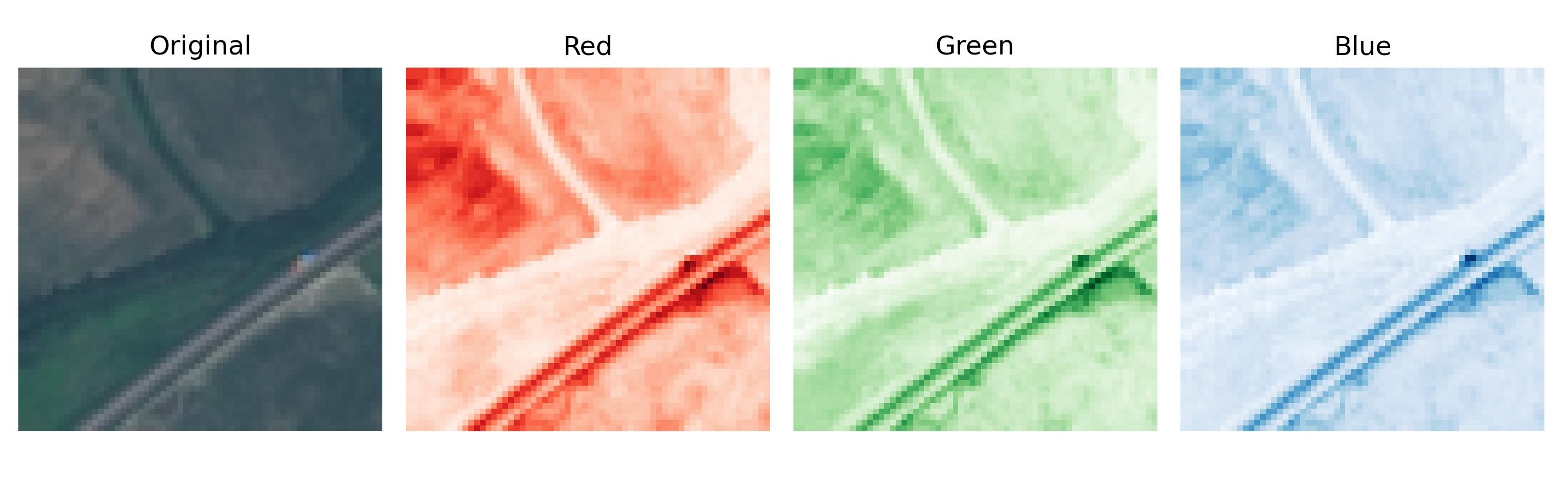
Data splitting
Before we train the models, we split the data into training (70%), validation (15%) and testing (15%).
split = [0.7, 0.15, 0.15]  # train, val, test
# this dictionary creates an id for each label
label2idx = {label: i for i, label in enumerate(label_names)}

# we store the filenames and labels in lists
files, targets = [], []
for label in label_names:
    label_files = glob(os.path.join(data_dir, label, "*.jpg"))
    files += label_files
    targets += [label2idx[label]] * len(label_files)

# we split the lists into training, validation, and test
train_files, temp_files, train_labels, temp_labels = train_test_split(
    files, targets, train_size=split[0], stratify=targets, random_state=1)

val_size = split[1] / (split[1] + split[2])  # proportion of val in temp
val_files, test_files, val_labels, test_labels = train_test_split(
    temp_files, temp_labels, train_size=val_size,
    stratify=temp_labels, random_state=1)
Training a “traditional” xgboost model
First, we try out “traditional” machine learning, or, more specifically, we train an xgboost model. The xgboost algorithm sequentially trains decision trees on the errors of the current ensemble of trees. The model that xgboost produces is an ensemble of trees.
When using traditional machine learning on image-like data, the question is always: What do we use as input features? In theory, we could flatten the 32x32x3 vector into a feature vector of length 3072, but that’s quite many features. Another option is to create new features from the input bands. This is the option I went for: For each RGB band, extract the mean values, the standard deviation, the minimum and the maximum.
Instead, we extract statistics from each of the input bands, namely the mean, the standard deviation, the minimum and the maximum.
def extract_features_from_path(img_path):
    img = Image.open(img_path).convert('RGB')
    arr = np.array(img)
    features = []
    for i in range(3):  # R, G, B
        ch = arr[:, :, i]
        features.append(ch.mean())
        features.append(ch.std())
        features.append(ch.min())
        features.append(ch.max())
    return features  # 12 features

X_train = np.array([extract_features_from_path(p) for p in train_files])
X_val   = np.array([extract_features_from_path(p) for p in val_files])
X_test  = np.array([extract_features_from_path(p) for p in test_files])

y_train = np.array(train_labels)
y_val   = np.array(val_labels)
y_test  = np.array(test_labels)

# For the xgboost model, we combine training and validation
X_trainval = np.concatenate([X_train, X_val])
y_trainval = np.concatenate([y_train, y_val])
Next, we train an xgboost model and tune the hyperparameters using randomized search via cross validation. This means we recombine the training and validation data and then repeatedly split the combined dataset into training and validation to tune the hyperparameters. The reason I split the data in the first place was for the neural network that we will train later.
# the parameters to sample from to try out
param_grid = {
    'n_estimators': [50, 100, 200, 500],
    'max_depth': [3, 5, 7, 9],
    'learning_rate': [0.01, 0.1, 0.2, 0.3],
    'subsample': [0.6, 0.8, 1.0],
}

clf = RandomizedSearchCV(XGBClassifier(eval_metric='mlogloss'),
                   param_grid, cv=5, scoring='accuracy', n_jobs=-1, verbose=1, n_iter=30)

clf.fit(X_trainval, y_trainval)
print("Best parameters:", clf.best_params_)
Fitting 5 folds for each of 30 candidates, totalling 150 fits
Best parameters: {'subsample': 0.6, 'n_estimators': 500, 'max_depth': 5, 'learning_rate': 0.1}
In total, the model tries out 30 (n_iter) hyperparameter configurations, sampled from param_grid. I opted for a five-fold cross-validation (cv), meaning the dataset is split repeatedly into 80% training and 20% validation data. Note that the test data was not part of that, so we still have a left-out dataset.
Next, we evaluate the model’s accuracy with this untouched test data.
y_pred = clf.predict(X_test)

acc = accuracy_score(y_test, y_pred)
precision, recall, f1, _ = precision_recall_fscore_support(y_test, y_pred, average='macro')

print(f"Accuracy:  {acc:.4f}")
print(f"Precision: {precision:.4f}")
print(f"Recall:    {recall:.4f}")
print(f"F1 score:  {f1:.4f}")
Accuracy: 0.8306
Precision: 0.8222
Recall: 0.8249
F1 score: 0.8229
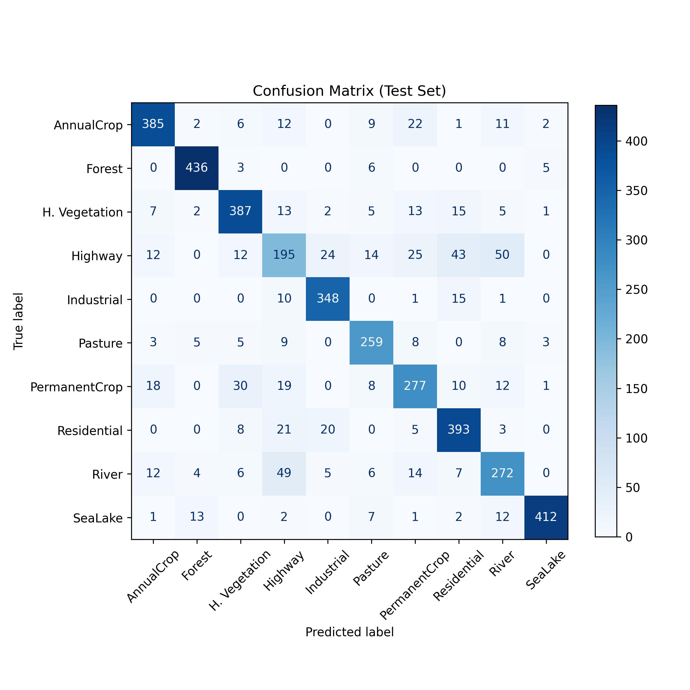
That’s way better than random classification already. Let’s see for which classes the model makes mistakes by visualizing the confusion matrix.
y_pred = clf.predict(X_test)
cm = confusion_matrix(y_test, y_pred)

short_labels = [ln.replace("HerbaceousVegetation", "H. Vegetation")
               for ln in label_names]
disp = ConfusionMatrixDisplay(confusion_matrix=cm, display_labels=short_labels)
fig, ax = plt.subplots(figsize=(8, 8))
im = disp.plot(ax=ax, cmap='Blues', xticks_rotation=45, colorbar=False)
cbar = fig.colorbar(im.im_, ax=ax, shrink=0.7)
plt.title('Confusion Matrix (Test Set)')
plt.tight_layout()
plt.savefig('./images/landcover-confusion-xgboost.jpg', dpi=300)
plt.show()
Figure 7.4 shows that the biggest weakness of the models are highways: they are often misclassified as rivers, residential areas or permanent crop. Also permanent crop is often misclassified, for example as herbaceous vegetation.
Let’s see whether we can get better results with a neural network.
Training a deep neural network: ResNet-18
For our deep learning approach, we train a ResNet-18 image classifier. ResNet-18 is a convolutional neural network. It’s more on the lightweight side of image recognition models, so a good choice for relatively quick training. Instead of training this architecture from scratch, we initialize it with the weights from a ResNet-18 trained on ImageNet. This means that the ResNet-18 model was pre-trained on 1000 classes on ImageNet. Since we only have 10 classes here, we have to adapt the final layer to accommodate this number. We can also decide whether to continue training the entire network or just the final (or a few) layers. Since satellite images are quite different from “ordinary” images like that of a dog, I decided training it completely.
device = torch.device("cuda" if torch.cuda.is_available() else "cpu")
weights = ResNet18_Weights.DEFAULT

model = resnet18(weights=weights)
batch_size = 16

# Replace the classifier (EuroSAT has 10 classes)
model.fc = nn.Linear(model.fc.in_features, 10)
model = model.to(device)
Next we initialize the data loaders. The data loader for the training data includes random transformations such as random flipping, both vertically and horizontally, as well as random rotations. The transformations help make the dataset larger and make the model more robust.
class EuroSATDataset(Dataset):
    def __init__(self, files, labels, transform=None):
        self.files = files
        self.labels = labels
        self.transform = transform

    def __len__(self): return len(self.files)

    def __getitem__(self, idx):
        image = Image.open(self.files[idx]).convert("RGB")
        if self.transform: image = self.transform(image)
        return image, self.labels[idx]


class RandomFixedRotation:
    def __init__(self, angles=[0, 90, 180, 270]):
        self.angles = angles

    def __call__(self, img):
        angle = random.choice(self.angles)
        return TF.rotate(img, angle)

train_transform = transforms.Compose([
    transforms.RandomHorizontalFlip(),
    transforms.RandomVerticalFlip(),
    RandomFixedRotation(),  # Only 90, 180, 270
    transforms.ToTensor(),
    # The ResNet is pretrained on ImageNet
    # these are the stats of the ImageNet data
    transforms.Normalize(mean=[0.485, 0.456, 0.406],
                         std=[0.229, 0.224, 0.225]),
])
val_transform = transforms.Compose([
    transforms.ToTensor(),
    transforms.Normalize(mean=[0.485, 0.456, 0.406],
                         std=[0.229, 0.224, 0.225]),
])

train_data = EuroSATDataset(train_files, train_labels, train_transform)
val_data = EuroSATDataset(val_files, val_labels, val_transform)
test_data = EuroSATDataset(test_files, test_labels, val_transform)

train_loader = DataLoader(train_data, batch_size=batch_size,
                          shuffle=True, num_workers=0)
val_loader   = DataLoader(val_data, batch_size=batch_size, num_workers=0)
test_loader  = DataLoader(test_data, batch_size=batch_size, num_workers=0)
With the data in place, it’s time to train the ResNet-18 model. Time to train the model now. The optimization criterion is the cross entropy loss, which is defined as:
\[CEL = \sum_{i=1}^n \sum_{c \in C} y^{(i)}_c log(f_c(x^{(i)}))\]
where \(y^{(i)}_c\) indicates whether data instance \(i\) is class c (\(y^{(i)}_c=1\)) or not (\(y^{(i)}_c=0\)) and \(f_c(x^{(i)}))\) is the model output for class c for data point \(i\) with features \(x^{(i)}\). We optimize the model with stochastic gradient descent with momentum.
learning_rate = 0.001
momentum = 0.9

# the loss function
criterion = nn.CrossEntropyLoss()
optimizer = optim.SGD(model.parameters(), lr=learning_rate, momentum=momentum)

def train_epoch(model, dataloader, optimizer, criterion):
    model.train()
    running_loss, correct, total = 0.0, 0, 0

    for inputs, labels in tqdm(dataloader, desc="Training", leave=False):
        inputs, labels = inputs.to(device), labels.to(device)

        optimizer.zero_grad()
        outputs = model(inputs)
        loss = criterion(outputs, labels)
        loss.backward()
        optimizer.step()

        running_loss += loss.item() * inputs.size(0)
        _, preds = torch.max(outputs, 1)
        correct += (preds == labels).sum().item()
        total += labels.size(0)

    return running_loss / total, correct / total

def evaluate(model, dataloader, criterion):
    model.eval()
    running_loss, correct, total = 0.0, 0, 0

    with torch.no_grad():
        for inputs, labels in dataloader:
            inputs, labels = inputs.to(device), labels.to(device)

            outputs = model(inputs)
            loss = criterion(outputs, labels)

            running_loss += loss.item() * inputs.size(0)
            _, preds = torch.max(outputs, 1)
            correct += (preds == labels).sum().item()
            total += labels.size(0)

    return running_loss / total, correct / total
The code above didn’t run the model training yet, but only defined the training and evaluation steps to take in each epoch. With the following lines, we finally train the model.
train_losses, train_accuracies = [], []
val_losses, val_accuracies = [], []

# Define the number of epochs
epochs = 30
# Number of epochs without improvement of validation loss for early stop
patience = 5
best_val_loss = float('inf')
patience_counter = 0

for epoch in range(epochs):
    train_loss, train_acc = train_epoch(model, train_loader, optimizer, criterion)
    val_loss, val_acc = evaluate(model, val_loader, criterion)

    train_losses.append(train_loss)
    train_accuracies.append(train_acc)
    val_losses.append(val_loss)
    val_accuracies.append(val_acc)

    print(f"Epoch {epoch+1}/{epochs}: "
          f"Train Loss {train_loss:.4f}, Acc {train_acc:.4f} | "
          f"Val Loss {val_loss:.4f}, Acc {val_acc:.4f}")
    # Early stopping logic
    if val_loss < best_val_loss:
        best_val_loss = val_loss
        patience_counter = 0
        torch.save(model.state_dict(), "best_model.pt")
    else:
        patience_counter += 1
        if patience_counter >= patience:
            break
Having trained the model, next we want to evaluate its performance. Figure 7.5 shows how the accuracy changes by epoch. We also evaluate the accuracy on the test data.
plt.figure(figsize=(12, 5))
plt.subplot(1, 2, 1)
plt.plot(train_losses, label='Train Loss')
plt.plot(val_losses, label='Val Loss')
plt.title('Loss over Epochs')
plt.xlabel('Epoch')
plt.ylabel('Loss')
plt.legend()

plt.subplot(1, 2, 2)
plt.plot(train_accuracies, label='Train Acc')
plt.plot(val_accuracies, label='Val Acc')
plt.title('Accuracy over Epochs')
plt.xlabel('Epoch')
plt.ylabel('Accuracy')
plt.legend()
plt.tight_layout()
plt.savefig("images/landcover-loss-curve.jpg", dpi=300)
plt.show()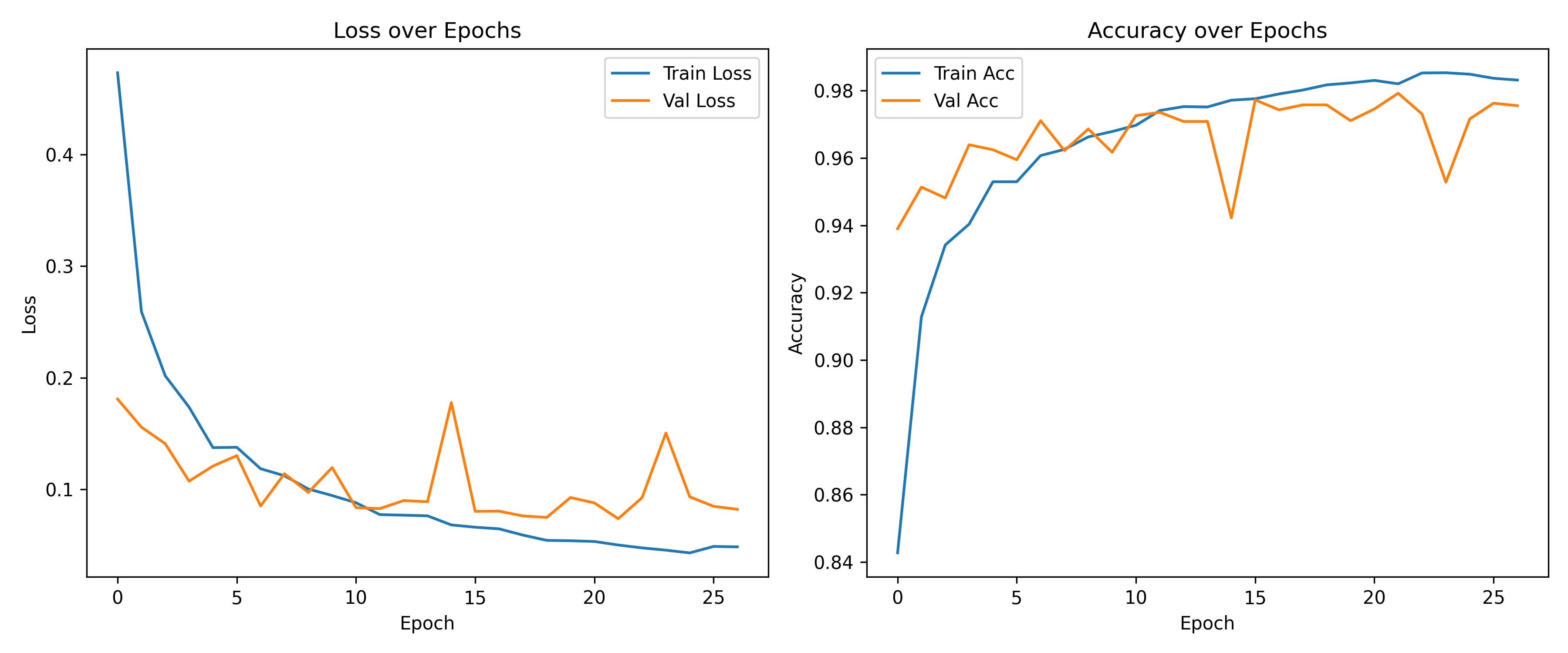
test_loss, test_acc = evaluate(model, test_loader, criterion)
print(f"Test Accuracy: {test_acc:.4f}")
Test Accuracy: 0.9733
As the Accuracy shows, the ResNet-18 model is much better than the xgboost. This doesn’t surprise me, as the convolutional neural networks are well-suited for image-like data. To be fair, the random forest could use some better features. We could introduce things like edge detectors, texture features, histogram-based features. Or we could divide the image into a grid and compute region-wise statistics. However, this is all what the convolutional layers are designed to learn on their own. If you want more interpretability in terms of these hand-crafted features traditional ML + satellite imagery is fine, but I would rather go, in this case, with the deep learning approach.
Figure 7.6 shows the mistakes that the model makes on the test data. Let’s look at the largest non-diagonal cells: Some permanent crop images were be misclassified as annual crop or herbaceous vegetation. Some rivers were misclassified as highways. But all in all, it’s a really strong model.
model.eval()

all_preds = []
all_labels = []

with torch.no_grad():
    for inputs, labels in test_loader:
        inputs = inputs.to(device)
        labels = labels.to(device)
        outputs = model(inputs)
        _, preds = torch.max(outputs, 1)
        all_preds.extend(preds.cpu().numpy())
        all_labels.extend(labels.cpu().numpy())
cm = confusion_matrix(all_labels, all_preds)
disp = ConfusionMatrixDisplay(confusion_matrix=cm, display_labels=short_labels)
fig, ax = plt.subplots(figsize=(8, 8))
disp.plot(cmap='Blues', xticks_rotation=45)
plt.title("Confusion Matrix on Validation Set")
plt.tight_layout()
plt.savefig("images/landcover-resnet-confusion.jpg", dpi=300)
plt.show()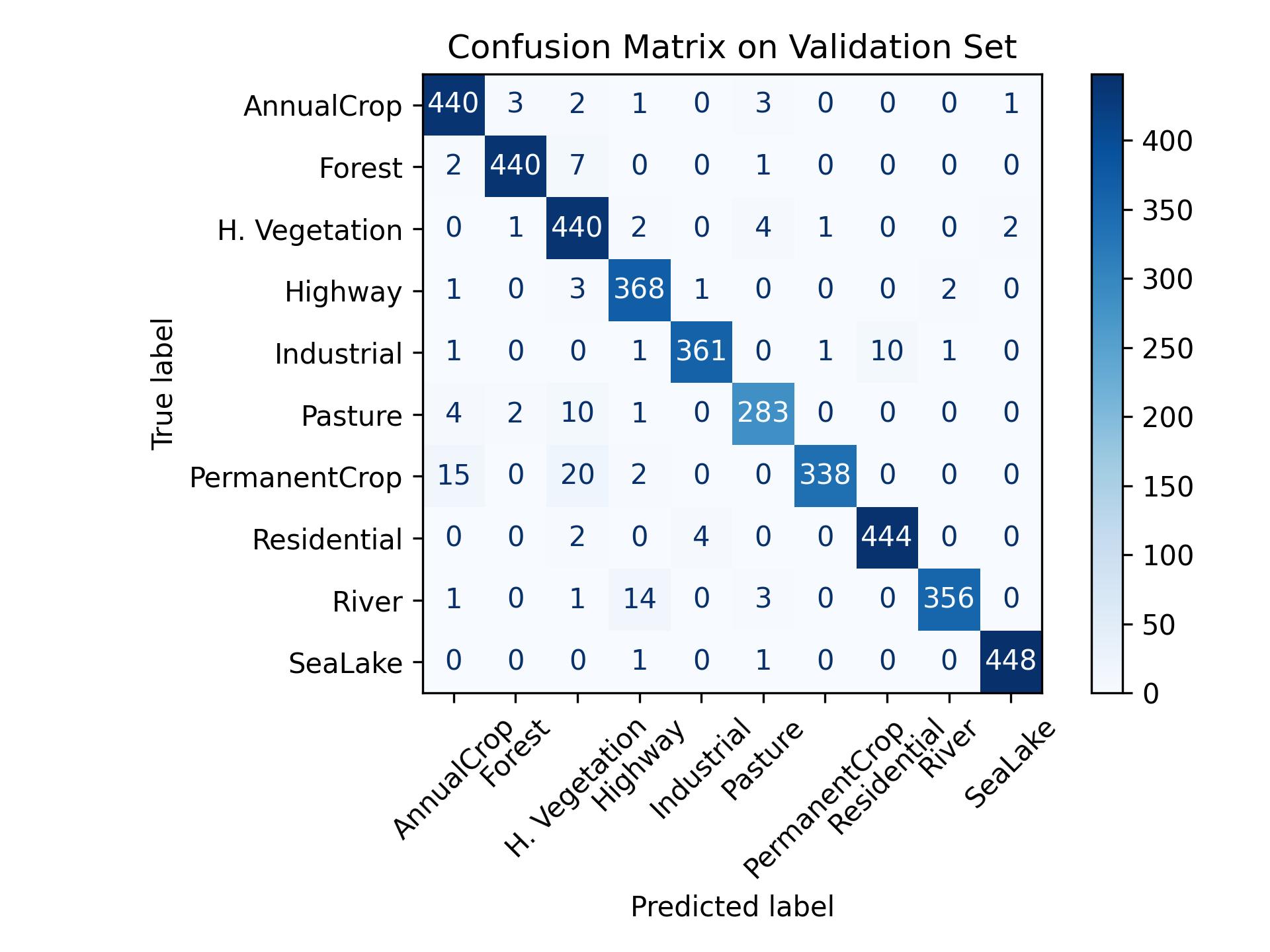
Limitations and further ideas
- The models only do image-wise classification. This is quite the limitation as there might be many classes visible in the satellite image.
- Multi-label classification might be another option, however this would need a differently labeled dataset.
- The models might still be useful in pre-filtering satellite data: For example, if you want to label images, you might use such a classifier to remove images that only show water.
But at least I don’t have the cite the Journal of Eugenics.↩︎