2 Coordinate Reference Systems (CRS)
In this chapter, you will:
- Understand what a Coordinate Reference System is and why we need it.
- Pick a suitable CRS for your machine learning application.
When working with satellite data, we need to know exactly where on Earth the image was taken. This is important when combining features and labels, when integrating satellite data with, for example, elevation models or ground sensor readings, and simply when interpreting the results in the real world.
Unfortunately, Earth isn’t flat. If it were flat, we could just describe any location using a simple 2D coordinate system. But it’s not. Earth is a geoid. It’s shaped like an oblated ellipsoid (because the rotation makes it bulge at the equator). In addition, valleys, mountains and oceans makes Earth bumpy, so that it’s final look is that of an anti-stress ball, see Figure 2.1. To make geographic computations manageable, we approximate Earth with an ellipsoid. And on this ellipsoid, we can define a coordinate system.

What is a Coordinate Reference System?
A coordinate reference system, short CRS, is a way to locate a point on Earth. A CRS is defined by three things: an ellipsoid model, a datum, and a projection method (optional).
An ellipsoid model of Earth is a smooth, mathematical approximation of Earth’s shape. This choice doesn’t matter as much for machine learning use cases.
A datum defines the center, positioning and orientation of the ellipsoid model relative to Earth. Since Earth isn’t a perfect ellipsoid, we have some freedom where to center the ellipsoid. The choice of datum influences how fine-grained we can reference different regions. We can distinguish between global and local datums:
- NAD 83, the North American Datum fits North America well.
- ETRS 89, the European Terrestial Reference System fits Europe well.
- WSG84, the World Geodetic System 1984 is a good compromise for all of Earth.
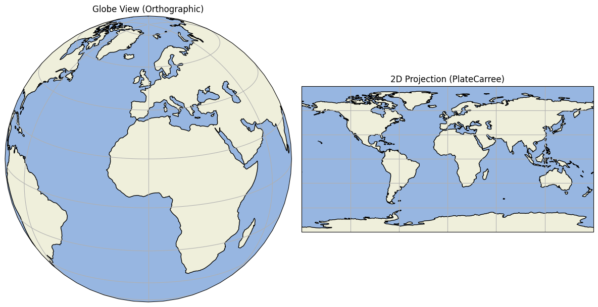
A projection method (optional) defines how to convert coordinates from the curved Earth to a flat 2D map. If you don’t use a projection, you have a geographic CRS using latitude (north-south angle) and longitude (east-west angle). For machine learning, it’s more common to use a projected CRS, which gives us a flat map (2D). Map projections always distort the images, and depending on which projection method you pick, you may preserve, for example, the area sizes, or distances, or angles, but never all of them at the same time. Projections can be: cylindrical, conic, azimuthal, and pseudocylindrical. An example of a cylindrical projection can be seen in Figure 2.2
Which CRS to pick for your project
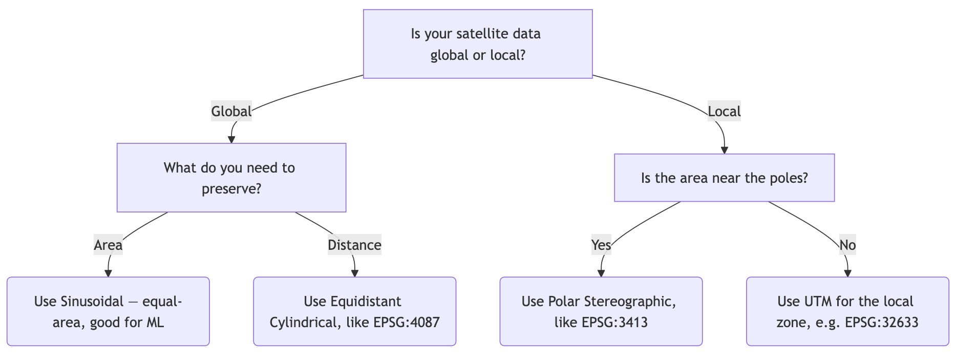
Let’s talk business: Which coordinate reference system should you pick for you machine learning application? Each has a different trade-off, so it really depends on the location of your satellite data images: Are they spread all over the world? Or are they mostly from a certain region, like the northern US? Is it important that, for example, the area is preserved? Figure 2.3 shows a very simplified decision tree for picking a Coordinate Reference System.
Warning
Avoid mixed projections across samples. Reproject everything to one system before modeling.
Checking and changing CRS in Python
We use the rioxarray library to load satellite data, check it’s current CRS and reproject it into a new one.
import rioxarray

raster = rioxarray.open_rasterio("data/satellite.tif")
print("Original CRS:", raster.rio.crs)

reprojected = raster.rio.reproject("EPSG:32633")
print("Reprojected CRS:", reprojected.rio.crs)
Original CRS: EPSG:4326
Reprojected CRS: EPSG:32633Note: EPSG:4326 is a geographic projection, useful for global datasets, GPS and web maps. EPSG:32633 is a projected CRS, with X and Y coordinates in meters. It approximately preserves distances, area, and direction so we could use it go calculate distance features, but only in the zone 33N, which covers central Europe.
We can also visualize the reprojected image:
import matplotlib.pyplot as plt

original_band = raster.isel(band=0)
reprojected_band = reprojected.isel(band=0)

fig, (ax1, ax2) = plt.subplots(1, 2, figsize=(10, 5))
ax1.imshow(original_band, cmap="gray")
ax1.set_title("Original")
ax1.axis("off")

ax2.imshow(reprojected_band, cmap="gray")
ax2.set_title("Reprojected")
ax2.axis("off")

plt.tight_layout()
plt.show()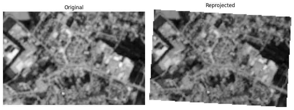
As you can see, the reprojection looks different and this highlights how mismatching CRS sources can introduce problems in the data.
Best Practice
- Pick a CRS that aligns with the region of the analyzed data.
- If you have different data sources, make sure they are projected into a common CRS before merging, otherwise they will mismatch. Also, project into a common CRS as early as possible in the pipeline.
- When calculating features like areas and distances, make sure to use a map projection that preserves the required property. For example, for area-preserving calculations, use an “equal-area projection” such as the sinusoidal projection.