8  Wildfire Spread Prediction

In this use case, we will predict how wildfires spread within 24 hours, using a U-NET neural network architecture.

A causal flick of a burning cigarette but; a dry forest; strong winds. A wildfire starts, hot enough to be detected by thermal satellites.

Where should the firefighters focus their attention? Which places have to be evacuated?

To decide these things, we have to predict where the fire will spread. Wildfire spread depends on many factors, like the extend of the initial fire, the dryness of the surrounding area, elevation and much more. A perfect use case for machine learning.

Designing the prediction task

How can we model wildfire spread with machine learning? When using satellites, we get a “fire” map, a binary map that says fire yes or no for each pixel. This requires some pre-processing, since thermal satellites measure heat on a scale, so we have to apply a threshold and remove false positives like burnings form industry plants (e.g., controlled burnings of methane). For this use case, however, the data pre-processing of the raw satellite images into binary fire maps is already done.

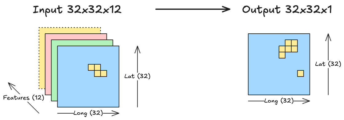
Since we are interested in modeling wildfire spread over time, we need binary fire maps for two points in time, for example, on day t and on day t+1. The fire map on t+1 is our outcome. So the prediction task looks like in Figure 8.1.

Example 1

Example 2

Figure 8.1: Two examples of wildfires in the Next Day Wildfire Spread data. The grey area is the fire on day t, the red area marks the fire at day t+1. Fires can persist.

However, we don’t only want to predict fire at t+1 from the fires at t, but use additional information, like the elevation profile, the wind strengths, the dryness, and so on. We can spatially represent this information as images of the same size as the fire map at time t.

This makes the input an “image” or rather a 3-dimensional tensor with the dimensions longitude, latitude, and features. A regular image typically has three features, like red, green, and blue channels, but we will work with many more. The prediction task itself can be seen as a segmentation task, because we segment our tensor into fire vs. no fire at time t+1, as visualized in Figure 8.2.

Figure 8.2

The “Next Day Wildfire Spread” data

To train a wildfire spread prediction model, we need data. Fortunately, there is already data available: Huot et al. (2022) collected and published the “Next Day Wildfire Spread” dataset. The dataset is published in multiple places, one being Kaggle. . It’s published with a CC-BY 4.0 license, meaning you are allowed to mix and adapt it, even use it commercially, as long as you attribute the authors.

The authors created the dataset with Google Earth Engine. Here is what’s inside the Next Day Wildfire Data:

• 18545 fire events across the US from 2012 to 2020.
• Each fire event has two snapshots, one at time t, one at t+1.
• Satellite images are 64 x 64 pixels, each representing 1km x 1km
• Inputs:
  • previous fire mask, elevation
  • wind direction
  • wind speed
  • min temp
  • max temp
  • humidity
  • precipitation
  • drought
  • vegetation
  • population density
  • energy release component
• Output: Wildfire on the next day.
• The fire events are split into training (80%), validation (10%) and testing (10%).

The dataset is hosted on Kaggle, but can be downloaded without an account. The following code snippet shows how to download and unzip the dataset. Just change the folder locations as needed.

curl -L -o ~/Downloads/next-day-wildfire-spread.zip\
  https://www.kaggle.com/api/v1/datasets/download/fantineh/next-day-wildfire-spread
unzip ~/Downloads/next-day-wildfire-spread.zip -d ~/Downloads/next-day-wildfire-spread

The files looks like this:

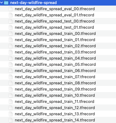
The file format .tfrecord is specific to the deep learning library TensorFlow.

Data preparation and augmentation

Thankfully, Huot et al. (2022) have published their code along with paper and data, so that I could build on that. They released their code in a Github repository under the Apache License 2.0, which allows commercial use as well. While I used their code as starting point, I made a lot of changes, but many of their modeling choice, like the way they did data augmentation, I kept.

First, let’s load all the necessary libraries for this use case:

import os
import re
from typing import Dict, List, Optional, Text, Tuple

import numpy as np
import matplotlib.pyplot as plt
from matplotlib.patches import Patch

import tensorflow as tf
from tensorflow.keras import layers, callbacks, optimizers
import keras

tf.random.set_seed(42)
np.random.seed(42)

Before loading the data, we define the feature names and feature scaling parameters. These were provided by Huot et al. (2022).

INPUT_FEATURES = [
    'PrevFireMask', 'elevation', 'th', 'vs', 'tmmn', 'tmmx', 'sph',
    'pr', 'pdsi', 'NDVI', 'population', 'erc'
]
OUTPUT_FEATURES = ['FireMask']
PREV_FIRE_MASK_INDEX = INPUT_FEATURES.index('PrevFireMask')

DATA_STATS = { # Format: (min_clip, max_clip, mean, std)
    'PrevFireMask': (-1.0, 1.0, 0.0, 1.0),
    'elevation': (0.0, 3141.0, 657.3, 649.0),
    'th': (0.0, 360.0, 190.3, 72.6),
    'vs': (0.0, 10.02, 3.85, 1.41),
    'tmmn': (253.15, 298.95, 281.1, 8.98),
    'tmmx': (253.15, 315.09, 295.2, 9.82),
    'sph': (0.0, 1.0, 0.0072, 0.0043),
    'pr': (0.0, 44.53, 1.74, 4.48),
    'pdsi': (-6.13, 7.88, -0.005, 2.68),
    'NDVI': (-9821.0, 9996.0, 5157.6, 2466.7),
    'population': (0.0, 2534.06, 25.53, 154.72),
    'erc': (0.0, 106.25, 37.33, 20.85),
    'FireMask': (-1.0, 1.0, 0.0, 1.0),
}

18k wildfire images is a good start, but for machine learning it’s not that many. A good way to improve this number without collecting more data is data augmentation. Figure 8.3 visualizes the 3 data augmentation steps of random cropping, random flipping, and random rotation. The random cropping steps randomly cuts out 32x32 chunks of the initial 64x64 tensors, both for the input and output of course. Random flipping is implemented to flip the image horizontally with a 50% change and also vertically with a new coin flip. Random rotation has a 25% for each of the following rotations: rotate by 0, 90, 180 or 270 degrees.

Figure 8.3: Data augmentation steps.

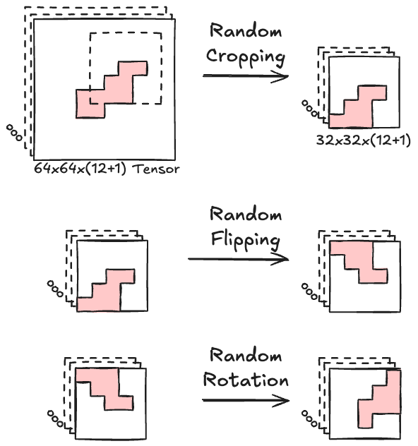
Besides increasing the number of images, data augmentation helps make the model more robust. For example, in the US the wind often blows from the west (the westerlies), so a model might learn a general rule that fires tend to spread to the east. By introducing random flipping, the model might be more prone to learn to follow the wind direction instead of learning a fixed “fire goes east” bias. Also, the way the data are collected, the fires are centered in the middle of the 64x64 images. I initially trained a model on the 64x64 data, and it had a strong bias to simply predict that the fires will remain there, since fires tend to persist. The random cropping makes the model actually learn to focus on areas where the fire started.

The following code implements the data reading, preparation, and augmentation:

# Removes extreme values and rescales to [-1;1]
def _clip_and_rescale(x: tf.Tensor, key: Text) -> tf.Tensor:
  min_val, max_val, _, _ = DATA_STATS[key]
  x = tf.clip_by_value(x, min_val, max_val)
  return (
    x if key == "PrevFireMask" else
    tf.math.divide_no_nan(x - min_val, max_val - min_val) * 2 - 1
  )

# Turns a data point into features+label
def _parse_fn(proto: tf.train.Example, size: int) -> Tuple[tf.Tensor, tf.Tensor]:
    keys = INPUT_FEATURES + OUTPUT_FEATURES
    parsed = tf.io.parse_single_example(proto, {
        k: tf.io.FixedLenFeature([size, size], tf.float32) for k in keys
    })
    x_features = [_clip_and_rescale(parsed[k], k) for k in INPUT_FEATURES]
    x = tf.stack(x_features, axis=-1)
    y_features = [parsed[k] for k in OUTPUT_FEATURES]
    y = tf.stack(y_features, axis=-1)
    return x, y

# Responsible for cropping, rotating, and flipping images randomly 
def _augment(x: tf.Tensor, y: tf.Tensor) -> Tuple[tf.Tensor, tf.Tensor]:
    combined = tf.concat([x, y], axis=-1)
    combined = tf.image.random_crop(combined, [32, 32, tf.shape(combined)[-1]])
    combined = tf.image.random_flip_left_right(combined)
    combined = tf.image.random_flip_up_down(combined)
    
    # Apply random 90° rotation: k ∈ {0, 1, 2, 3}
    k = tf.random.uniform([], minval=0, maxval=4, dtype=tf.int32)
    combined = tf.image.rot90(combined, k)

    in_ch = len(INPUT_FEATURES)
    return combined[..., :in_ch], combined[..., in_ch:]

def _has_fire(x: tf.Tensor, y: tf.Tensor) -> tf.Tensor:
    has_prev_fire = tf.reduce_any(tf.equal(x[..., PREV_FIRE_MASK_INDEX], 1.0))
    not_all_masked = tf.reduce_any(tf.not_equal(y, -1.0))
    return tf.logical_and(has_prev_fire, not_all_masked)


# Data set generator
def get_dataset(split: Text, batch_size=64, size=64) -> tf.data.Dataset:
    filenames = f"data/next-day-wildfire-spread/next_day_wildfire_spread_{split}*"
    files = tf.data.Dataset.list_files(filenames)
    return (files
        .interleave(tf.data.TFRecordDataset, num_parallel_calls=tf.data.AUTOTUNE)
        .map(lambda x: _parse_fn(x, size), num_parallel_calls=tf.data.AUTOTUNE)
        .shuffle(16000)
        .map(_augment, num_parallel_calls=tf.data.AUTOTUNE)
        .filter(_has_fire)
        .batch(batch_size)
        .prefetch(tf.data.AUTOTUNE))

The _clip_and_rescale function makes sure that the data doesn’t take on extreme values and makes sure the data is between -1 and +1. Due to the random cropping, images without a fire at time t can be introduced. The filter step makes sure that these are removed from the data, since they have no value for training a wildfire spread prediction model.

Finally, we can use the function get_dataset to generate the training, validation, and test datasets.

train_dataset = get_dataset('train')
validation_dataset = get_dataset('eval')
test_dataset = get_dataset('test')

Training the U-Net model

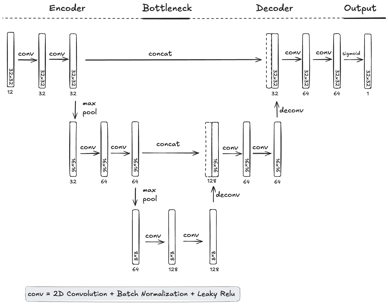
I decided to train a U-Net architecture (Ronneberger, Fischer, and Brox 2015), which is a classic choice for segmentation tasks. U-Nets consist of an encoder, a bottleneck, a decoder part, and an output layer. The job of the encoder is to distill information from the features, the job of the decoder to scale it again to an image. During encoding, information gets spatially coarser. The bottleneck forces the model to learn condensed features. In addition, U-Net architectures have skip-layer connections, meaning previous, more raw layer information “survives” the encoding and is concatenated in the decoding part with the information pushed through the bottleneck. The skip layer part is the right inductive bias for wildfire spread prediction, since especially the wildfire mask at time t is an important feature for which we want to keep the spatial resolution high. The last layer is a sigmoid layer, which means that we get an 32x32 image with values between 0 and 1. Visualizing this architecture as in Figure 8.4, it’s useful to arrange the layers in a U-form to highlight these skip-connections, hence the name U-NET.

The typical U-Net is one pooling/deconvolution step deeper. However, the images in the bottleneck would then be 4x4, which would be very coarse, so I opted for a more shallow version with an 8x8 resolution bottleneck. Also, I trained the model on my notebook, so a more shallow U-Net made that faster.

Figure 8.4: A (shallow) U-Net architecture that I used for predicting wildfire spread.

# Convolutional block for U-NET
def conv_block(x, filters):
    for _ in range(2):
        x = layers.Conv2D(filters, 3, padding='same')(x)
        x = layers.BatchNormalization()(x)
        x = layers.LeakyReLU(0.1)(x)
    return x

# Designing the U-NET Architecture
def build_unet(input_shape=(32, 32, 12)):
    inputs = tf.keras.Input(shape=input_shape)                 # (32, 32, 12)

    # Encoder
    enc1 = conv_block(inputs, 32)                              # (32, 32, 32)
    pool1 = layers.MaxPooling2D()(enc1)                        # (16, 16, 32)

    enc2 = conv_block(pool1, 64)                               # (16, 16, 64)
    pool2 = layers.MaxPooling2D()(enc2)                        # (8, 8, 64)

    # Bottleneck
    bottleneck = conv_block(pool2, 128)                        # (8, 8, 128)

    # Decoder
    up2 = layers.Conv2DTranspose(64, 3, strides=2, padding='same')(bottleneck)#(16, 16, 64)
    concat2 = layers.Concatenate()([up2, enc2])                # (16, 16, 128)
    dec2 = conv_block(concat2, 64)                             # (16, 16, 64)

    up1 = layers.Conv2DTranspose(32, 3, strides=2, padding='same')(dec2)#(32, 32, 32)
    concat1 = layers.Concatenate()([up1, enc1])                # (32, 32, 64)
    dec1 = conv_block(concat1, 32)                             # (32, 32, 32)

    outputs = layers.Conv2D(1, 1, activation='sigmoid')(dec1)  # (32, 32, 1)

    return tf.keras.models.Model(inputs, outputs)

Next, we define the loss function that we optimize the U-Net for. I picked the binary focal loss (Lin et al. 2020), which is defined as:

\[ \text{FL}(p_t) = -\alpha_t (1 - p_t)^\gamma \log(p_t), \]

where \(p_t\) is the model’s estimated probability for the true class, \(\alpha_t\) is a weighting factor, and \(\gamma\) is a focusing parameter that reduces the loss contribution from easy examples and extends it for hard ones.

The focal loss is particularly useful for imbalanced data. In our case, most pixels are “No Fire”. Only around ~1-2% of the pixels are classified as “Fire” at time t+1. The focal loss puts more weight on the difficult to classify examples, here the “Fire” events.

I didn’t use the TensorFlow implementation of the focal loss (tf.keras.losses.BinaryFocalCrossentropy), but used a custom one. The reason: there can be missing values in the output fire mask (with value = -1), which should be ignored when computing the loss. As Lin et al. (2020) recommended, I set \(\gamma=2\) – a good value for very imbalanced data – and left the default value of \(\alpha=0.25\) (this parameter is less important).

@tf.keras.utils.register_keras_serializable()
def masked_focal_loss(y_true: tf.Tensor, y_pred: tf.Tensor) -> tf.Tensor:
    mask = tf.cast(tf.not_equal(y_true, -1), tf.float32)
    bfc = tf.keras.losses.BinaryFocalCrossentropy(from_logits=False, gamma=2.0,
                                                  reduction=tf.keras.losses.Reduction.NONE)
    fl = bfc(y_true, y_pred)
    fl = tf.expand_dims(fl, -1) if fl.shape.rank == 3 else fl
    return tf.reduce_sum(mask * fl) / tf.reduce_sum(mask)

While we optimize for the focal loss, we want to evaluate the model on a different metric. For segmentation, one such metric is the area under the precision-recall curve (PR AUC).

It’s defined as the area under the curve that plots precision (positive predictive value) against recall (true positive rate) for different classification thresholds.
Formally, it’s the integral:

\[ \text{PR AUC} = \int_0^1 \text{Precision}(r) \, dr \approx \sum_{i=1}^{n-1}(r_{i+1} - r_{i})\cdot \frac{p_i + p_{i+1}}{2} \]

where \(r_i\) is the recall at point \(i\) and \(p_i\) the precision at point \(i\).

There are many more non-fire pixels than fire pixels in the outcome. That’s why we need a metric that is sensitive to this unbalanced outcome, which PR AUC is well suited for. Further, the PR AUC is a metric that is independent from the classification threshold that we use for classifying fire versus no-fire. This is especially useful if we want the model to be usable with different thresholds and also for visualizing the prediction gradually.

@tf.keras.utils.register_keras_serializable()
class MaskedPRAUC(tf.keras.metrics.AUC):
    def __init__(self, **kwargs):
        kwargs.setdefault('name', 'masked_pr_auc')
        kwargs.setdefault('curve', 'PR')
        super().__init__(**kwargs)

    def update_state(self, y_true, y_pred, sample_weight=None):
        mask = tf.not_equal(y_true, -1)
        y_true_masked = tf.boolean_mask(y_true, mask)
        y_pred_masked = tf.boolean_mask(y_pred, mask)
        return super().update_state(y_true_masked, y_pred_masked)

model = build_unet()
model.compile(
    optimizer=optimizers.Adam(1e-3),
    loss=masked_focal_loss,
    metrics=[MaskedPRAUC()]
)

In addition, I implemented early stopping in combination with reducing the learning rate when the validation loss plateaus.

early_stop = callbacks.EarlyStopping(monitor='val_masked_pr_auc', patience=5,
                                     restore_best_weights=True, mode='max')
reduce_lr = callbacks.ReduceLROnPlateau(monitor='val_masked_pr_auc', factor=0.5,
                                        patience=3, mode='max', verbose=1)

Now we can finally train the model:

history = model.fit(
    train_dataset,
    validation_data=validation_dataset,
    epochs=100,
    callbacks=[early_stop, reduce_lr],
)

The model training stops after 20 epochs due to the early stopping criteria. Figure 8.5 shows the AUC PR development over the epochs. Looking at the curve for the validation data, we can see that even after a few epochs (around 12), the model’s performance is almost saturated.

plt.figure(figsize=(8, 5))
plt.plot( history.history['masked_pr_auc'], label='Train PR AUC')
plt.plot(history.history['val_masked_pr_auc'], label='Validation PR AUC')
plt.xlabel('Epoch')
plt.ylabel('PR AUC')
plt.xticks([0, 5, 10, 15, 20])
plt.legend()
plt.grid(True)
plt.tight_layout()
plt.savefig('./images/wildfire_pr_auc.png', dpi=300)
plt.close()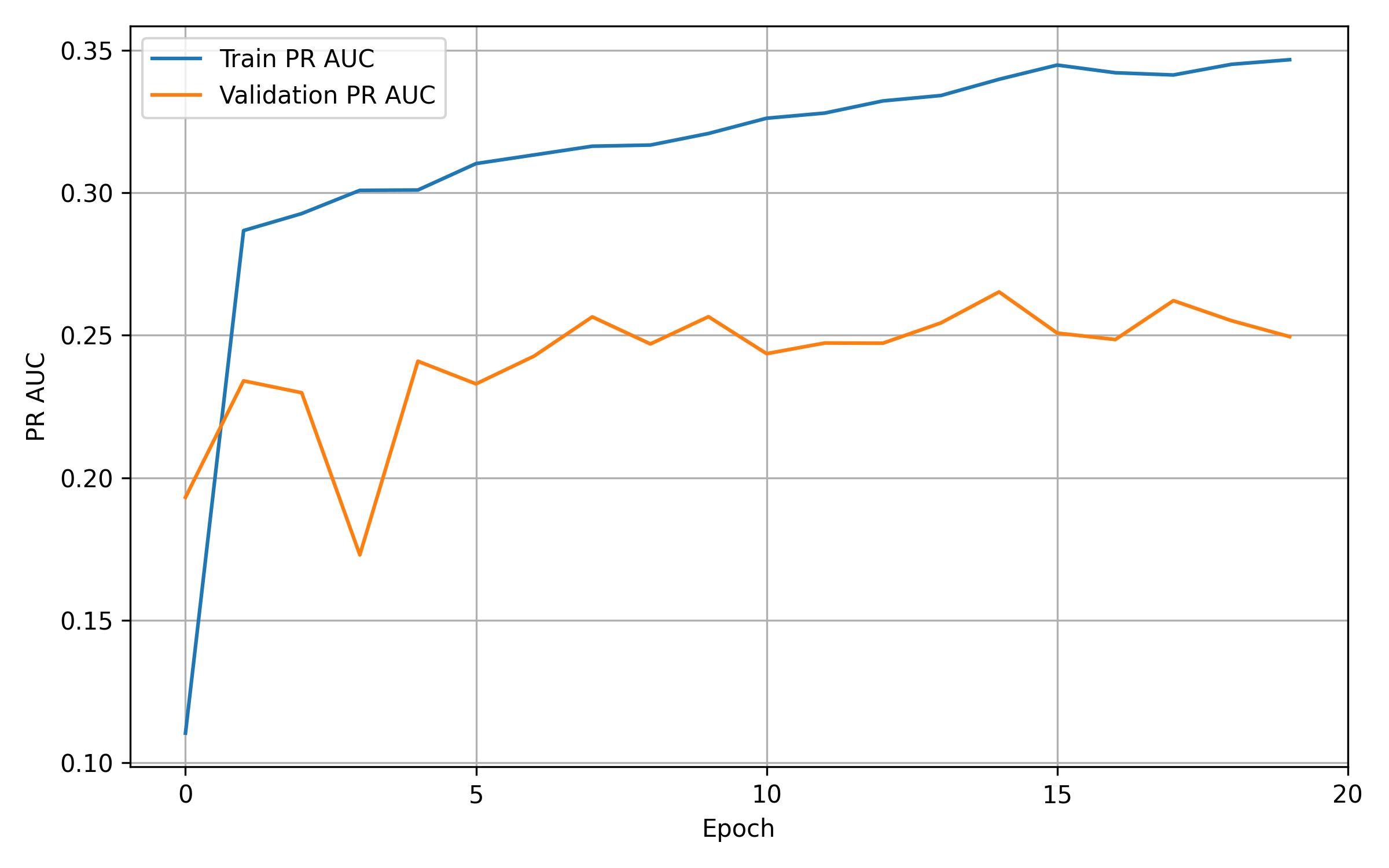

Figure 8.5: Training and validation PR AUC development by epoch.

Evaluating the Model

We still have the 10% test_dataset left, which we can use to evaluate the performance of the model. For the test data, I also compute the PR AUC. To get a feeling for how well the model works, I compare it with the “persistence” baseline, which simply predicts that the fire from time t will persist until time t+1.

# Force batches once into memory; Makes it deterministic
test_batches = list(test_dataset)
pr_auc_unet = MaskedPRAUC()
pr_auc_persistence = MaskedPRAUC()

# Iterate through test batches
for x_batch, y_batch in test_batches:
    y_pred = model.predict(x_batch, verbose=0)
    pr_auc_unet.update_state(y_batch, y_pred)
    y_persist = x_batch[:, :, :, PREV_FIRE_MASK_INDEX:PREV_FIRE_MASK_INDEX+1]
    valid_mask = tf.logical_and(y_batch != -1, y_persist != -1)
    y_persist_valid = tf.boolean_mask(y_persist, valid_mask)
    y_batch_valid = tf.boolean_mask(y_batch, valid_mask)
    pr_auc_persistence.update_state(y_batch_valid, y_persist_valid)


print(f"PR AUC UNET: {pr_auc_unet.result().numpy():.2f}")
print(f"PR AUC persistence baseline: {pr_auc_persistence.result().numpy():.2f}")

PR AUC UNET: 0.31

PR AUC persistence baseline: 0.16

A side note here: Computing the PR AUC for the persistence baseline is a bit of an edge case, since the persistence baseline only has 1’s and 0’s, so there is only one threshold for which to compute the curve with. But it can still serve as a rough comparison.

We can reuse the PR AUC object to compute precision and recall. Otherwise we would have to implement custom classes as well to deal with the missing values for wildfire at t+1.

tp = pr_auc_persistence.true_positives.numpy()
fp = pr_auc_persistence.false_positives.numpy()
fn = pr_auc_persistence.false_negatives.numpy()

# Precision and recall at each threshold
precision = tp / (tp + fp + 1e-8)
recall = tp / (tp + fn + 1e-8)

# result is a vector with different "cutoffs", which for the persistence baseline are mostly the same
# so picking just the 10th
print(f"Precision for persistence baseline: {precision[10]:.2f}")
print(f"Recall for persistence baseline: {recall[10]:.2f}")

Precision for persistence baseline: 0.40

Recall for persistence baseline: 0.29

If we want to compute precision and recall for our U-Net, we have to pick a threshold at which we would say it’s a fire or not. To be honest, I wouldn’t know which one to pick. Because the choice of threshold depends on the cost of false positive (saying fire but there’s none) versus false negative (predicting ‘no fire’ but there is one). That’s why I also picked the PR AUC to monitor the model: It’s a threshold-independent metric.

Let’s have a look at the precision-recall curve to figure out the relation between precision and recall here. Figure 8.6 shows how the U-Net performs.

tp = pr_auc_unet.true_positives.numpy()
fp = pr_auc_unet.false_positives.numpy()
fn = pr_auc_unet.false_negatives.numpy()

precision = tp / (tp + fp + 1e-8)
recall = tp / (tp + fn + 1e-8)

step = 20 # Select every 20th threshold
precision_sub = precision[::step]
recall_sub = recall[::step]
thresholds_sub = pr_auc_unet.thresholds[::step]

plt.plot(recall, precision, label=f"AUC = {pr_auc_unet.result().numpy():.3f}")
for r, p, t in zip(recall_sub, precision_sub, thresholds_sub):
    plt.plot(r, p, 'o', color='black', markersize=3)  # add a small dot
    plt.annotate(f't={t:.2f}', (r, p),
                 fontsize=8, ha='center', xytext=(0, 6), textcoords="offset points",
                 bbox=dict(boxstyle="round", fc="white", ec="0.7", alpha=0.8))

plt.xlabel("Recall")
plt.ylabel("Precision")
plt.title("Precision-Recall Curve")
plt.grid(True)
plt.legend()
plt.savefig('./images/wildfire_pr_curve.png', dpi=300)
plt.close()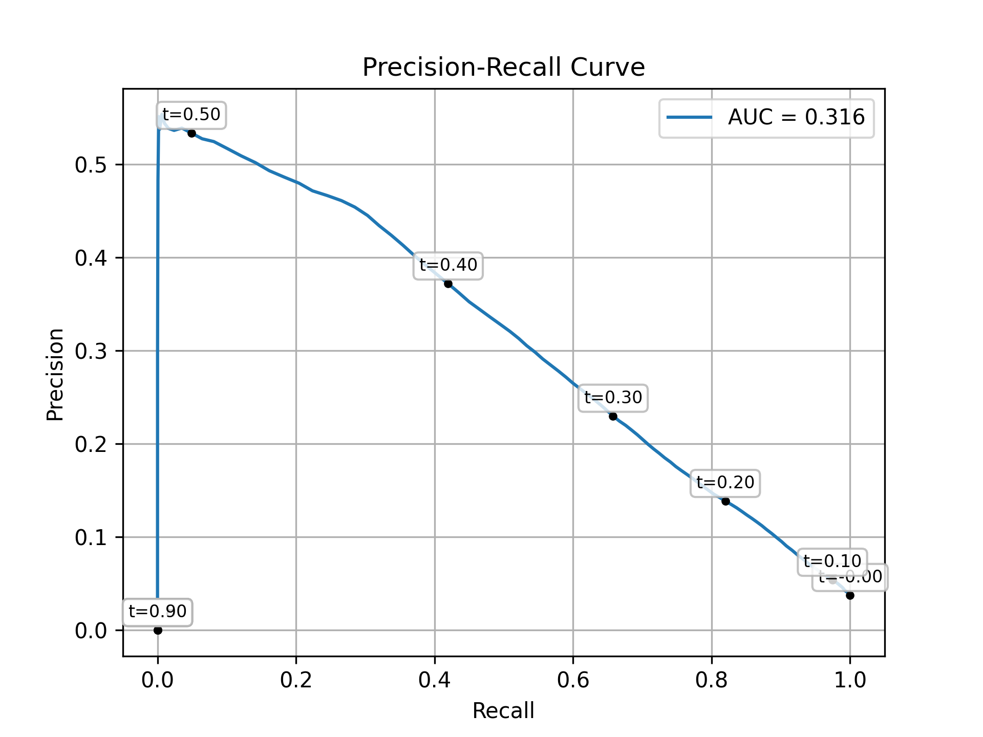

Figure 8.6: The precision-recall curve for the U-Net.

The area under the curve is 0.316, which is great! It’s comparable to the original paper (PR AUC of 28.4 for a ResNet autoencoder). This is quite neat, since we are using a simpler architecture without hyperparameter optimization, except for early stopping.

From this plot we can also read out precision and recall for different classification thresholds. If we would say that every pixel with a model score of >0.40 is a fire, we would get a precision of ~37% and a recall of ~42%. For a threshold of 0.5 we would get a precision of ~53%, but a really bad recall of ~.5%.

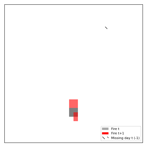
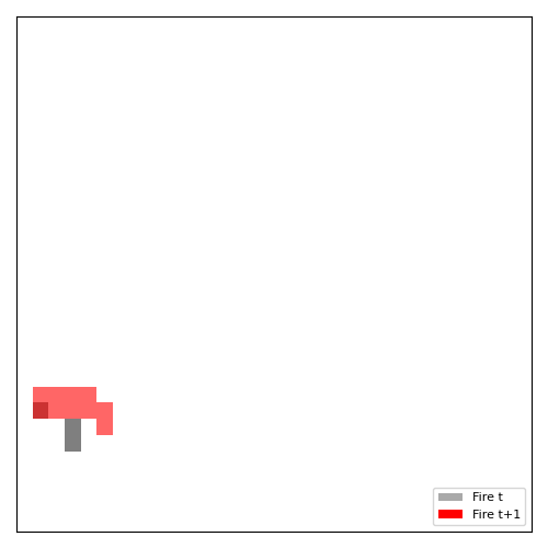
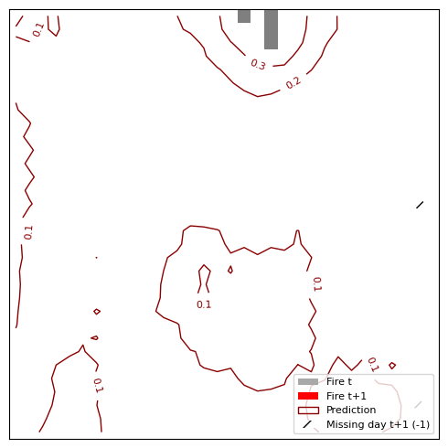
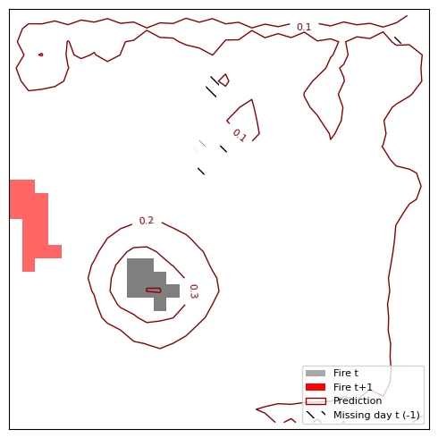
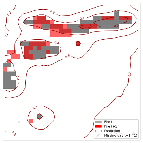
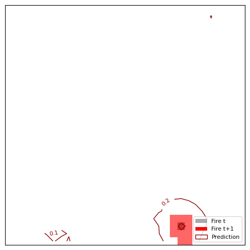
In addition to the aggregated metrics, let’s visualize a few cases so we get a feel for what the model predictions are like.

def plot_fire_prediction(x, y_true, y_old, y_pred=None):
    fig, ax = plt.subplots(figsize=(5, 5))
    y_t = np.where(y_old[..., None] == 1, [0.5, 0.5, 0.5, 1], [0, 0, 0, 0])
    ax.imshow(y_t, interpolation='none')
    y_t1 = np.where(y_true[..., None] == 1, [1, 0, 0, 0.6], [0, 0, 0, 0])
    ax.imshow(y_t1, interpolation='none')
    legend = [
        Patch(facecolor='darkgrey', label='Fire t'),
        Patch(facecolor='red', label='Fire t+1'),
    ]
    
    if y_pred is not None:
        cs = ax.contour(y_pred, levels=[0.1, 0.2, 0.3, 0.4, 0.5], colors='darkred', linewidths=1)
        ax.clabel(cs, inline=True, fontsize=8, fmt="%.1f")
        legend.append(Patch(facecolor='none', edgecolor='darkred', label='Prediction'))

    if np.any(y_true == -1):
        ax.contourf(y_true == -1, levels=[0.5, 1.5],colors='none', hatches=['//'])
        legend.append(Patch(facecolor='white', hatch='//', label='Missing day t+1 (-1)'))

    if np.any(y_old == -1):
        ax.contourf(y_old == -1, levels=[0.5, 1.5],colors='none', hatches=['\\\\'])
        legend.append(Patch(facecolor='white', hatch='\\\\', label='Missing day t (-1)')) 

    ax.legend(handles=legend, loc='lower right', fontsize=8)
    ax.axis('off')
    plt.tight_layout()
    return fig

The following code visualizes a few examples of predictions:

all_samples = []
for x_batch, y_batch in test_batches:
    preds = model(x_batch).numpy()

    for i in range(len(x_batch)):
        y_true = y_batch[i, :, :, 0].numpy()
        y_pred = preds[i, :, :, 0]
        pr_auc = MaskedPRAUC()
        pr_auc.update_state(y_true, y_pred)
        all_samples.append({
            'pr_auc': pr_auc(y_true, y_pred),
            'x': x_batch[i],
            'y_true': y_true,
            'y_old': x_batch[i][:, :, 0],
            'y_pred': y_pred
        })

# Sort samples by PR AUC
all_samples.sort(key=lambda s: s['pr_auc'])

# Pick a few examples
selected_samples = [
    ('bad', all_samples[0]),
    ('bad2', all_samples[200]),
    ('mid', all_samples[len(all_samples) // 2]),
    ('good', all_samples[-1])
]

# Plot and save
for label, sample in selected_samples:
    fig = plot_fire_prediction(sample['x'], sample['y_true'],
                               sample['y_old'], sample['y_pred'])
    fig.savefig(f"images/wildfire_prediction_{label}.png", bbox_inches='tight')
    plt.close(fig)

The resulting Figure 8.7 shows 4 predictions. In general, the model works well when the fires stay close to their original location and don’t spread too far. It doesn’t work so well for fires that no longer burn the next day or when fires “jump” from one location to another. One problematic thing might be the cropping: We can have the case that there is a large fire on the bottom. But random cropping yields only the part above and we get a small fire at the bottom of our 32x32 image. On the next day it seems that the fire jumped from bottom left to bottom right, but in reality it might be just an extension of the large fire that we cropped away from the bottom.

Wildfire prediction where the model doesn’t perform well.

Another wildfire prediction where the model underperforms

An Ok-ish prediction.

Here the wildfire spread model works well.

Figure 8.7: Different wildfire spread predictions. Grey areas show fire at time t, red areas the fire at time t+1. Fires can persist (darkred). The contour lines show the predicted fire spread.

Limitations and improvements

Just a few thoughts on how to use the model, and what can be improved:

• The model can be used to predict next day’s wildfire spread, which can be useful for making decisions of evacuation and where to focus fire fighting. Of course, I wouldn’t recommend using this toy example directly in production.
• One thing we ignored mostly was the threshold for classifying whether a pixel is fire or not. This involves finding a trade-off between precision and recall. However, that’s something that you can only decide in the context of an actual application in collaboration with the experts and/or users.
• I didn’t tune the model at all, so there might be room to improve the model by doing architecture search and tuning batch sizes etc.
• The current evaluation is a bit wonky: There is a huge discrepancy between the PR AUC on validation and on test data. To get more stable results, you could use cross-validation, especially since the model only takes a few minutes to train.

Huot, Fantine, R. Lily Hu, Nita Goyal, Tharun Sankar, Matthias Ihme, and Yi-Fan Chen. 2022. “Next Day Wildfire Spread: A Machine Learning Dataset to Predict Wildfire Spreading From Remote-Sensing Data.” IEEE Transactions on Geoscience and Remote Sensing 60: 1–13. https://doi.org/10.1109/TGRS.2022.3192974.

Lin, Tsung-Yi, Priya Goyal, Ross Girshick, Kaiming He, and Piotr Dollár. 2020. “Focal Loss for Dense Object Detection.” IEEE Transactions on Pattern Analysis and Machine Intelligence 42 (2): 318–27. https://doi.org/10.1109/TPAMI.2018.2858826.

Ronneberger, Olaf, Philipp Fischer, and Thomas Brox. 2015. “U-Net: Convolutional Networks for Biomedical Image Segmentation.” In Medical Image Computing and Computer-Assisted Intervention–MICCAI 2015: 18th International Conference, Munich, Germany, October 5-9, 2015, Proceedings, Part III 18, 234–41. Springer.