3  Remote Sensing Indices

Satellite sensors record their images in bands such as red, green, blue, and near-infrared. If you are interested in particular metrics, like understanding how much vegetation there is, there isn’t one “vegetation” band ¹, but the information may be spread across bands.

The solution is to compute indices from the bands which best represent the information for things like vegetation, to soil, and urban development. Remote sensing indices are mathematical formulas that involve two or more bands. The indices are computed on a pixel-level, so the outcome of computing this for an entire satellite image would be again the size of that image. And we can overlay it to see the image in a “different light”.

There’s hundreds if not thousands of these indices. For a full overview, I recommend the website indexdatabase.io. In this chapter, I’ll give you just two examples, an index for vegetation (NDVI) and one for urban areas (NDBI).

As an example, we’ll use this image from Mayrhofen in Austria Figure 3.1. I downloaded the image from https://browser.dataspace.copernicus.eu/. You need an account, but it’s free.

The following code simply reads in the image and visualizes it with red, green, and blue color channels.

import rasterio
import numpy as np
import matplotlib.pyplot as plt

def load_bands(paths):
    return [rasterio.open(p).read(1) for p in paths]

paths = ['./data/mayrhofen/B04.jpg',  # Red band
         './data/mayrhofen/B03.jpg',  # Green band
         './data/mayrhofen/B02.jpg',  # Blue band
         './data/mayrhofen/B08.jpg',  # Near-infrared band
         './data/mayrhofen/B11.jpg']  # Short-wave infrared band 

red, green, blue, nir, swir = load_bands(paths)
rgb = np.dstack([red, green, blue])

plt.figure(figsize=(8, 8))
plt.imshow(rgb)
plt.title("RGB Image (Sentinel-2)")
plt.axis('off')
plt.show()

Figure 3.1: Satellite image of Mayrhofen, Austria from July 17th, 2025 captured by Sentinel-2A.

Compute vegetation with NDVI

Use the Normalized Difference Vegetation Index (NDVI) to assess health and density of vegetation.

The formula to compute NDVI is:

\[\text{NDVI} = (\text{NIR} - \text{Red}) / (\text{NIR} + \text{Red})\]

So first we compute the difference in intensity between near infrared and red bands. Then we divide the difference by the combined intensity. The more vegetation there is in the image, the less red there will be as plants absorb the red color, but they reflect the near infrared waves.

Table 3.1: Interpretation of NDVI values. Note that such thresholds are a bit arbitrary and not super scientific.

NDVI	Interpretation
<0	Water, snow, clouds
0.0 – 0.1	Bare soil, sand, rock
0.1 – 0.2	Sparse vegetation (e.g. shrubs, grass)
0.2 – 0.5	Moderate vegetation (e.g. cropland, grassland)
0.5 – 0.7	Dense vegetation (e.g. temperate forests)
0.7 - 1.0	Very dense vegetation (e.g. tropical rainforests)

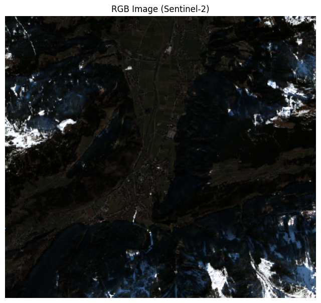
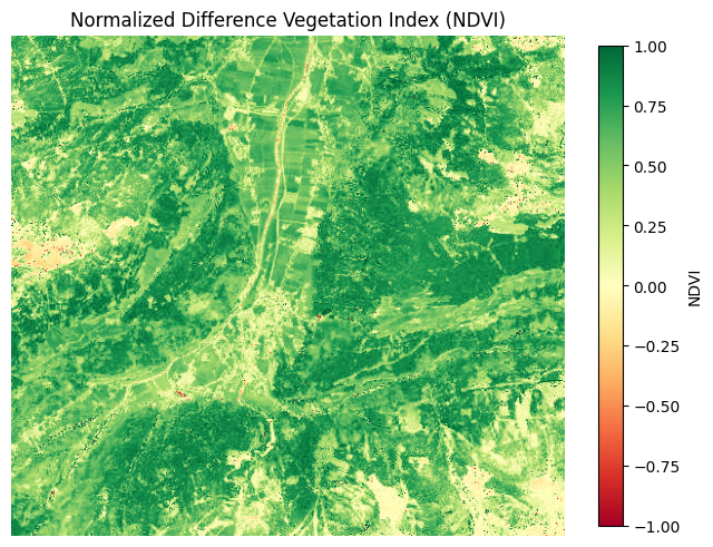
For Figure 3.2 I computed the NDVI for the image prior in this chapter. The greener the color, the more dense the vegetation in the pixel. Note that, different from RGB bands, there is no “true” color that NDVI has, so we are free to pick something. Green makes sense for high values of NDVI, but keep in mind that it doesn’t represent the green light, although it’s highly correlated with green plants, of course. Things like urban areas, water, and snow have a 0 or even negative NDVI.

ndvi = (nir.astype(float) - red.astype(float)) / (nir + red + 1e-10)

plt.figure(figsize=(8, 8))
plt.imshow(ndvi, cmap='RdYlGn', vmin=-1, vmax=1)
plt.colorbar(label='NDVI', shrink=0.7)
plt.title("Normalized Difference Vegetation Index (NDVI)")
plt.axis('off')
plt.show()

Figure 3.2: NDVI version of Mayrhofen from Figure 3.1.

Detect urban areas with NDBI

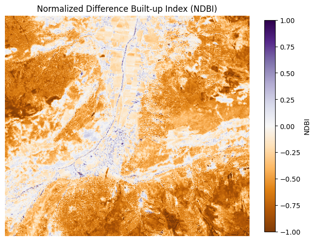
The Normalized Difference Built-up Index (NDBI) can be used to detect structures built by humans. It uses short-wave infrared and near-infrared bands:

\[\text{NDBI} = (\text{SWIR} - \text{NIR}) / (\text{SWIR} + \text{NIR})\]

Buildings reflect lots of short-wave infrared and less near-infrared. For vegetation, it’s the opposite. That’s why positive values of NDBI may be interpreted as buildings and streets. Note that also mountains and other bare land can have a high NDBI.

Tip

Indexes starting with an N usually are “Normalized” meaning they are scaled to -1 and 1.

Figure 3.3 shows the NDBI for Mayrhofen. Things like roads and buildings get a large NDBI while, e.g., vegetation gets a negative value. Note that, the Sentinel-2A’s SWIR band (B11) normally has a 20m resolution while the other bands have 10m. However, this was already resampled to the 10m scale before downloading the data.

ndbi = (swir.astype(float) - nir.astype(float)) / (swir + nir + 1e-10)

plt.figure(figsize=(8, 8))
plt.imshow(ndbi, cmap='PuOr', vmin=-1, vmax=1)
plt.colorbar(label='NDBI', shrink=0.7)
plt.title("Normalized Difference Built-up Index (NDBI)")
plt.axis('off')
plt.show()

Figure 3.3: NDBI version of Mayrhofen from Figure 3.1.

Find indices for a known sensor

Many of the indices require specific wavelengths. This means, depending on which sensors your data come from, you might or might not be able to actually compute the value. Let’s say you have already settled on imagery from the Sentinel-2A satellite. Which indexes can you use in this case? Fortunately, there is a simple way to find out:

1. Go to indexdatabase.io
2. Select the sensor you work with and click Display Indices
3. The site gives you a list of indices suitable for the sensor output.

Warning

Not all indices can be computed from all satellites. Check beforehand whether a satellite sensor records the relevant bands!

How to use indices for machine learning

In machine learning, indices can be used as input features (aka feature engineering). Depending on your prediction task, you add these indices as features to your input data. For example, for crop type classification, you might compute the NDVI and add it as a feature to your input data. Depending on your modeling approach, especially when using deep learning, you might not need these indices, since they do not contain any new information if you already use the respective bands as features in your model. Deep learning models tend to learn their own features, so you can just try it out whether you really need indices. Indices may still improve interpretability and generalization.

---

1. At first glance, the green might seem useful or even sufficient for vegetation,, right? Since plants absorb red and blue light, but reflect green light. However, there are other things that emit green light, like algae, and there is more information in other bands like near-infrared.